Stochastic versus deterministic effects

Tom Breur

13 February 2019

Building reliable analytical models requires separating signal from noise. When Machine Learning (ML) algorithms pursue an exhaustive search for patterns that relate an array of input variables to your target variable, random fluctuations can easily (seem to) ‘cause’ spurious relationships. I use quotation marks because predicting is something principally different from explaining, as Galit Shmueli has eloquently pointed out. Machine Learning is usually employed for prediction, not explanation.

Not all “signal” that gets detected by your ML algorithm is created equal, the topic of this blog post. Signal can originate from stochastic or deterministic effects, the latter often a thorny source of undesirable variation. Data quality issues can wreak havoc, and can be caused in various ways. This distinction is an important and particularly tricky one. Mitigating artefacts like deterministic sources of variation is one of the finer points in predictive model building.

But before I go into the nitty gritty details about stochastic versus deterministic effects, let’s clarify what you can and cannot learn by partitioning your model set (see: Berry & Linoff, Mastering Data Mining, 1999), the records that include your labeled target class that we use to develop predictive models.

 

Causal confounding

When you divide your dataset into a training and a test partition, this helps to isolate signal from the noise. Or rather: you equip yourself to empirically verify the stability (some say “robustness”) of your findings. If you discover a pattern in the training data, and can reproduce that same phenomenon in the test data (that you never touched to discover the pattern), you have additional reassurance that effect upholds – at least in this data sample.

Note however, that partitioning only helps you determine robustness of findings within your dataset. In no way whatsoever (!!) does splitting your dataset into train and test data safeguard you against erroneous conclusions as a result of (causal) “leakers” (Berry & Linoff, 1997), sometimes also referred to as “anachronistic variables.” Personally, I find the latter a much more descriptive term. To my knowledge it was introduced by Dorian Pyle in 1999.

Leakers or anachronistic variables are present in exactly the same way in both partitions: your training and you test data. Therefore, no amount of cross-validation can surface this problem! The problem of causal leakers only becomes apparent after you deploy your model in the real world. That’s when the predictive modeler learns the hard way about “causal confounding”: the model performs (often much) worse in real life than anticipated on the basis of patterns in the training and test data sets. It’s the proverbial “egg on your face” for predictive modelers. Because variation in your input array is caused by rather than predictive for the target variable, there is confounding of predictors and the target variable.

Just like with anachronistic variables, troublesome variation that is caused by deterministic effects, will appear in exactly the same way in both (all) partitions of your model set.

 

Surfacing stochastic effects

Now that we have distinguished the thorny problem of “causal confounding”, “anachronistic variables”, I would like to turn to the ‘real’ topic of this blog post: stochastic versus deterministic effects. I consider predictive modeling the killer app for data science, and therefore some sort of taxonomy of anti-patterns needs to be thoroughly understood. Unwanted deterministic effects are –unfortunately– often less pronounced, and can be (much) harder to detect than anachronistic variables. If your predictive model sinks like a led balloon once it gets deployed, there will be little doubt something went terribly wrong. For stochastic versus deterministic effects the magnitude is often (much) less pronounced, and therefore you face more of a risk that it will linger on. Just like with anachronistic variables, troublesome variation as a result of deterministic effects will appear in exactly the same way in all your model set partitions.

 

What to do about these challenges?

The obvious next question becomes: “what to do about these effects?” One of the lessons I picked up from my time in the trenches, is that ‘real’ signals, can sometimes be notoriously hard to pick up. This got me wondering. There can be several reasons why “signals” (real effects) get buried in a sea of screeching noise. The distinction between stochastic and deterministic effects has really “stuck” with me after building thousands of models. Fake or spurious associations (“deterministic effects”) tend to “jump out” more prominently than legitimate effects. What do I mean by that?

Human behavior is inherently difficult to predict. We sometimes behave erratically, have free will, and different people can respond to the same stimulus in different ways. This creates a substantial amount of genuinely ‘random’ variance. As a result, you can hardly expect predictive models to have super high accuracy, because that would imply our behavior is highly consistent and governed by transparent observable rules that can be accurately captured in mathematical equations. If you buy into the notion of free will, it becomes evident why conspicuously strong (univariate) effects should always give cause for concern. Stochastic effects are caused by “real” (human) variance, deterministic effects are an artefact of the data propagation process. An example of this would be something “minor” like truncating fractions at two digits behind the comma, or something more obviously problematic like replacing NULL values with zero.

After you build a model, it is common practice to run a so-called “sensitivity analysis” on the array of variables that made it into the eventual model. When you order the variables from most important to least important, what you expect to find is a more or less gradual decline in importance. Any and all of the variables that have a markedly higher association than others merit further inspection. How are they related to the target variable? What does this variable measure? How is this data field generated? How does it relate to the target variable, as well as other variables? Strong multi-collinearity (also with variables not included in the final model) can pose a serious threat to stability of the model.

Suppose we plot the relationship between the target variable and all the input variables in our model, and it looks something like this:

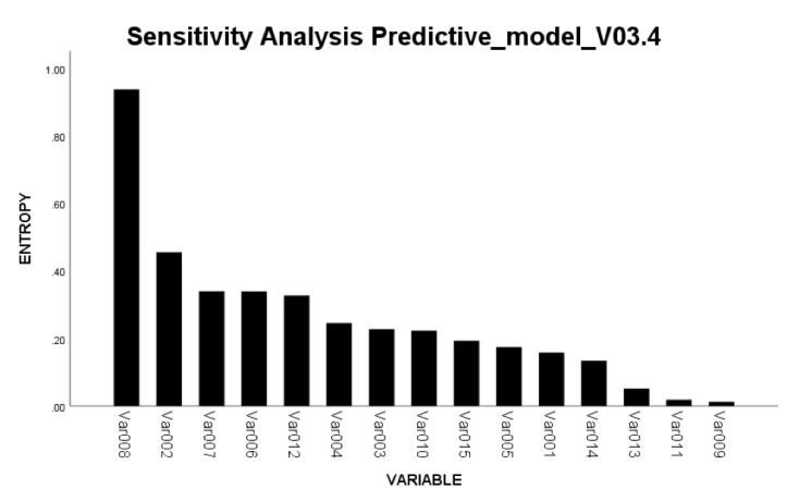
This shows a sensitivity plot very much just like it might appear in real life. Some people like to use statistical p-value on the Y-axis, in this diagram Entropy was used because it is better suited to (also) capture non-linear associations. My first thought now is going to be: how come Var008 is such a strong predictor?!? The association seems about twice as strong as the second best variable, and that gives food for thought. Especially now that all the others seem largely in the same range. Very suspicious.

Sometimes there genuinely is one variable much more important for prediction than others. That is when a chart like this one might occur. However, much more often when I see a chart with a distribution like this, there turns out to be some systematic effect embedded in either data capture, or the data transformation process. This is why I consider it an artefact of data propagation. Maybe certain values got truncated, but for the “wrong” reasons. “It seemed such a good idea, at the time” I have heard all too often. Maybe there was some hidden bias in data collection? An ETL artefact? Etc., etc.

There seems no limit to the number of ways data can trip you up. You can rarely take them at face value. Somehow, they never ever seem to be what they appear. Some examples of deterministic effects I have run into myself:

• NULL values got replaced with zero. It seemed reasonable at the time, but introduced undesirable bias because of the systematic pattern of zeros and NULLs.
• Outlier records were removed because they “messed up” the model. But what if these records represent a genuine effect? This becomes an even thornier issue in in a sparsely populated variable. This is a very real problem, much like outliers in insurance claims data are as much statistical outliers as they represent the genuine effect actuaries want to model! There aren’t many claims against the insurance, and most of them are small to moderate. Yet the big ones are the insurance company’s main risk.
• Values of categories were grouped, or continuous variables binned, in ways that obfuscated valuable patterns.

Here is an example of a deterministic effect. Once I was working with a dataset from a financial services company. Because they carried so many products, every individual customer held only a relatively small subset of those products. Now imagine I do not hold an investment account, should my value then be coded as NULL, or zero? Obviously the former, but in order to make processing more convenient, data engineers had “helped” by recoding all NULL values to zero. It was indeed easier to process like this, but as a side effect, this operation had “equated” customers with zero balance with those who didn’t hold the product at all…

There is no end to the number of ways that data extraction, pulling together datasets across disparate source systems, or data preparation for that matter can introduce spurious patterns in a modeling data set. Likewise for the subtle ways data extraction tactics can obfuscate important patterns. And once these “design choices” are welded into the dataset, they become deterministic effects that are genuinely present in the data. Since they do not relate to actual customer behavior. Any signal they convey can be highly misleading to the unwary data scientist.

 

Conclusion

The common denominator among all these deterministic effects I have mentioned is that they create a systematic impact on the relation between input variables and the output. Hence my use of the term “deterministic” effect. Because (“genuine”) human behavior is stochastic in nature, the “crisp” patterns that deterministic relations create tends to show a notably stronger association than stochastic patterns from genuine human behavior.

When variables “stand out” and show a strikingly higher association with your target variable, this phenomenon might be at play. But unfortunately, the deterministic patterns can also be subtle, and lurking in the midst of “average” variables that comprise a valid reflection of discretionary human behavior. When the systematic effect only impacts a (small) subset of records, this problem may not be so clear at all.

There is no substitute for a profound understanding of how data are generated by the underlying primary business processes. This is a (yet another) case for explaining your model (see an earlier post on “Three reasons why you always need to explain your model”), to tap into shared understanding of the data propagation processes, to give yourself a better chance that at least someone in the team will pick up a spurious deterministic effect.